library(tidyverse)EPA - EDA 3
Packages
Data
We’ll be using another version of the EPA PM2.5 data used in the the previous EPA - EDA pages. This version has been modified and saved locally in several csv files.
- pm0 contains data from 1999
- pm1 contains data from2012
- cnames.txt is a variable containing list of characters for column names
- wcol_df is a df holds the indices of the 5 columns we
- site0 and site1 are for sensors in the NY state area for 1999 and 2012 respectively described as County.Code and Site.ID concatenated together with “.” as seperator
Save csv & txt files
List of the files and how they were saved
if(!file.exists("D:/yourdataiq/dataiq/datasets/pm0.csv"))
        {write_csv(pm0,"D:/yourdataiq/dataiq/datasets/pm0.csv")}
if(!file.exists("D:/yourdataiq/dataiq/datasets/pm1.csv"))
        {write_csv(pm1,"D:/yourdataiq/dataiq/datasets/pm1.csv")}
if(!file.exists("D:/yourdataiq/dataiq/datasets/cnames.csv"))
        {writeLines(cnames,"D:/yourdataiq/dataiq/datasets/cnames.txt")}
if(!file.exists("D:/yourdataiq/dataiq/datasets/wcol.csv"))
        {write_csv(wcol_df,"D:/yourdataiq/dataiq/datasets/wcol.csv")}
if(!file.exists("D:/yourdataiq/dataiq/datasets/site0.csv"))
        {writeLines(site0,"D:/yourdataiq/dataiq/datasets/site0.txt")}
if(!file.exists("D:/yourdataiq/dataiq/datasets/site1.csv"))
        {writeLines(site1,"D:/yourdataiq/dataiq/datasets/site1.txt")}
Load
pm0 <- read.csv("D:/yourdataiq/dataiq/datasets/pm0.csv")
pm1 <- read.csv("D:/yourdataiq/dataiq/datasets/pm1.csv")
cnames <- readLines("D:/yourdataiq/dataiq/datasets/cnames.txt")
wcol_df <- read.csv("D:/yourdataiq/dataiq/datasets/wcol.csv")
site0_ <- readLines("D:/yourdataiq/dataiq/datasets/site0.txt")
site1_ <- readLines("D:/yourdataiq/dataiq/datasets/site1.txt")
Tidy
Case Study
We were given an index of the columns we will use in wcol
We were given a complete list of column names in cnames
So we need to extract the names from cnames corresponding to the wcol indices and assign to the column names of pm0
Let’s look at some of the data and cnames
dim(pm0)[1] 117421 5head(pm0) V1 V2 V3 V4 V5
1 1 27 1 19990103 NA
2 1 27 1 19990106 NA
3 1 27 1 19990109 NA
4 1 27 1 19990112 8.841
5 1 27 1 19990115 14.920
6 1 27 1 19990118 3.878make.names
- We were given a df of the columns we will use wcol
- We were given column names in cnames
- So we need to extract the names from cnames for only the wcol columns and assign to the names of the df pm0
cnames # is a list of 1 : chr[1] "# RD|Action Code|State Code|County Code|Site ID|Parameter|POC|Sample Duration|Unit|Method|Date|Start Time|Sample Value|Null Data Code|Sampling Frequency|Monitor Protocol (MP) ID|Qualifier - 1|Qualifier - 2|Qualifier - 3|Qualifier - 4|Qualifier - 5|Qualifier - 6|Qualifier - 7|Qualifier - 8|Qualifier - 9|Qualifier - 10|Alternate Method Detectable Limit|Uncertainty"strsplit
- It appears the column names are separated by |, so let’s split the vector by | and get the column names only. With
fixed=TRUEwe are asking to match | exactly. - Since we had to convert cnames to df to save it, we can no longer use the following code because cnames is now a df.
- So in the next line of code we convert the df to string then apply strsplit to it
cnames_stripped <- strsplit(cnames,"|", fixed = TRUE)
cnames_stripped
[[1]]
[1] "# RD" "Action Code"
[3] "State Code" "County Code"
[5] "Site ID" "Parameter"
[7] "POC" "Sample Duration"
[9] "Unit" "Method"
[11] "Date" "Start Time"
[13] "Sample Value" "Null Data Code"
[15] "Sampling Frequency" "Monitor Protocol (MP) ID"
[17] "Qualifier - 1" "Qualifier - 2"
[19] "Qualifier - 3" "Qualifier - 4"
[21] "Qualifier - 5" "Qualifier - 6"
[23] "Qualifier - 7" "Qualifier - 8"
[25] "Qualifier - 9" "Qualifier - 10"
[27] "Alternate Method Detectable Limit" "Uncertainty" Now that we have the column names as we want. Let’s look at which columns we need, so let’s look at wcol
wcol_df wcol
1 3
2 4
3 5
4 11
5 13convert wcol_df to vector
wcol_vector <- wcol_df[[1]]
wcol_vector
[1] 3 4 5 11 13make.names 1
Make syntactically valid names out of character vectors.
Syntax
make.names(names, unique = FALSE, allow_ = TRUE)names |
character vector to be coerced to syntactically valid names. This is coerced to character if necessary. |
unique |
logical; if TRUE, the resulting elements are unique. This may be desired for, e.g., column names. |
allow_ |
logical. For compatibility with R prior to 1.9.0. |
Let’s build this in two pieces:
- The code below will take the list of cnames_stripped and extract the wcol positions which are (3,4,5,11,13) and leaves us with a list of names for the desired columns
- The second block of code assigns the list to the colnames of the df: pm0_w_names
- So let’s copy pm0 to pm0_wnames first, to preserve the original df, and then perform our code
pm0_wnames <- pm0
head(pm0_wnames)
V1 V2 V3 V4 V5
1 1 27 1 19990103 NA
2 1 27 1 19990106 NA
3 1 27 1 19990109 NA
4 1 27 1 19990112 8.841
5 1 27 1 19990115 14.920
6 1 27 1 19990118 3.878cnames_stripped[[1]][wcol_vector][1] "State Code" "County Code" "Site ID" "Date" "Sample Value"make.names
names(pm0_wnames) <- make.names(cnames_stripped[[1]][wcol_vector])
head(pm0_wnames)
State.Code County.Code Site.ID Date Sample.Value
1 1 27 1 19990103 NA
2 1 27 1 19990106 NA
3 1 27 1 19990109 NA
4 1 27 1 19990112 8.841
5 1 27 1 19990115 14.920
6 1 27 1 19990118 3.878make names 2
Let’s do it without using make.names.
Let’s add colnames to the pm0 and save it in named_pm0
named_pm0 <- pm0
names(named_pm0) <- cnames_stripped[[1]][wcol_vector]
head(named_pm0)
State Code County Code Site ID Date Sample Value
1 1 27 1 19990103 NA
2 1 27 1 19990106 NA
3 1 27 1 19990109 NA
4 1 27 1 19990112 8.841
5 1 27 1 19990115 14.920
6 1 27 1 19990118 3.878NOTE
Do you notice the difference between named_pm0 and pm0_wnames? The latter was created with make.names which creates Systactically Valid Names (meaning: A syntactically valid name consists of letters, numbers and the dot or underline characters and starts with a letter or the dot not followed by a number. Names such as “.2way” are not valid, and neither are the reserved words.)
So notice the “.” in the column names.
make.names pm1
Let’s repeat the steps we used for pm0 but for pm1 instead and we end up with pm1_wnames
pm1_wnames <- pm1
head(pm1_wnames)
V1 V2 V3 V4 V5
1 1 3 10 20120101 6.7
2 1 3 10 20120104 9.0
3 1 3 10 20120107 6.5
4 1 3 10 20120110 7.0
5 1 3 10 20120113 5.8
6 1 3 10 20120116 8.0names(pm1_wnames) <- make.names(cnames_stripped[[1]][wcol_vector])
head(pm1_wnames) State.Code County.Code Site.ID Date Sample.Value
1 1 3 10 20120101 6.7
2 1 3 10 20120104 9.0
3 1 3 10 20120107 6.5
4 1 3 10 20120110 7.0
5 1 3 10 20120113 5.8
6 1 3 10 20120116 8.0EDA
2008 data
General Research
Column to vector
Assign Sample.Value column to a numeric vector with 117421 length and with NAs
x0 <- pm0_wnames$Sample.Value
str(x0)
num [1:117421] NA NA NA 8.84 14.92 ...Percent NAs
mean(is.na(x0)) # a little over 11%[1] 0.11256082012 data
General Research
Column to vector
x1 <- pm1_wnames$Sample.Value
str(x1)
num [1:1304287] 6.7 9 6.5 7 5.8 8 7.9 8 6 9.6 ...Percent NAs
mean(is.na(x1)) # a little over 5%[1] 0.05607125Summary
summary(x0) Min. 1st Qu. Median Mean 3rd Qu. Max. NA's
0.00 7.20 11.50 13.74 17.90 157.10 13217 summary(x1) Min. 1st Qu. Median Mean 3rd Qu. Max. NA's
-10.00 4.00 7.63 9.14 12.00 908.97 73133 Observations:
- Both mean and median decreased
- NA’s increased tremendously
- Negative values appeared in the data?
Negative values
- Assign negative values to a vector
- Count the occurences out of the 1.3+Million observations
- Of course we can calculate the % but let R do it using the mean once again: 2.1%
negative <- x1<0
sum(negative, na.rm = TRUE)
[1] 26474mean(negative, na.rm = TRUE)[1] 0.0215034head(negative)[1] FALSE FALSE FALSE FALSE FALSE FALSE- We can ignore the negative values, but let’s dig into it a bit more, maybe there are certain months the negative values occur?
- Let’s look at the Date column
Integer to date
str(pm1_wnames$Date) int [1:1304287] 20120101 20120104 20120107 20120110 20120113 20120116 20120119 20120122 20120125 20120128 ...pm0_wnames$Date <- as.Date(as.character(pm0_wnames$Date), "%Y%m%d")
pm1_wnames$Date <- as.Date(as.character(pm1_wnames$Date), "%Y%m%d")
str(pm0_wnames$Date) Date[1:117421], format: "1999-01-03" "1999-01-06" "1999-01-09" "1999-01-12" "1999-01-15" ...str(pm1_wnames$Date) Date[1:1304287], format: "2012-01-01" "2012-01-04" "2012-01-07" "2012-01-10" "2012-01-13" ...histogram of negatives
hist(pm1_wnames$Date[negative],"day",main="Negative readings per day")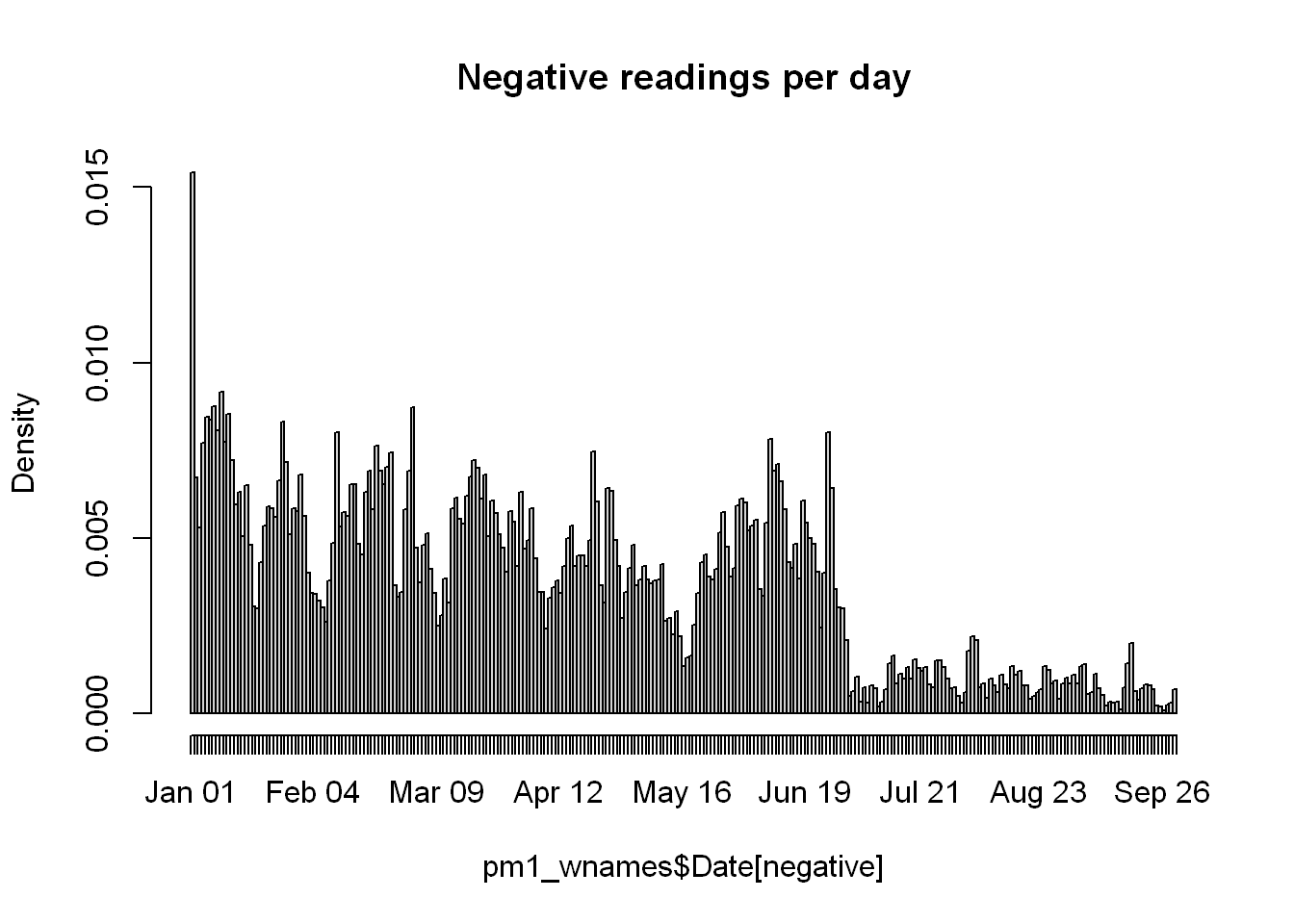
hist(pm1_wnames$Date[negative],"month",main="Negative readings per month")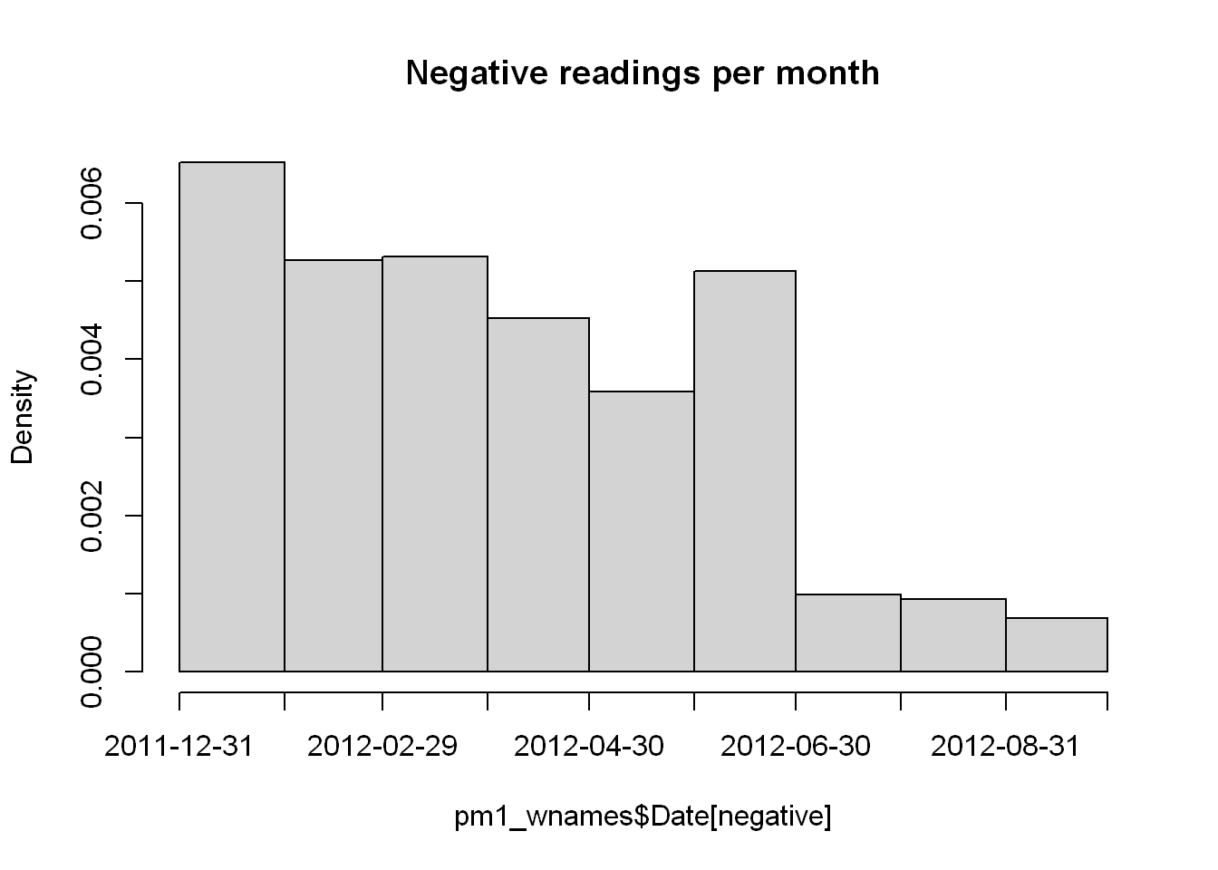
Common sensors
Let’s find common sensors between 1999 and 2012 and compare the values to see what we can find. - As noted from the Data section: site0 is for 1999 NY state sensors - site1 is for 2012 NY state sensors - Let’s look at the makeup of the data with str()
str(site0_) chr [1:33] "1.5" "1.12" "5.73" "5.80" "5.83" "5.110" "13.11" "27.1004" ...str(site1_) chr [1:18] "1.5" "1.12" "5.80" "5.133" "13.11" "29.5" "31.3" "47.122" ...Intersect
- Let’s find the intersect of both 1999 and 2012
- Data shows 10 monitors are still in use in 2012
both <- intersect(site0_,site1_)
both
[1] "1.5" "1.12" "5.80" "13.11" "29.5" "31.3" "63.2008"
[8] "67.1015" "85.55" "101.3" Paste two columns
Let’s concatenate both County.Code and Site.ID columns into one: we call it county.site, with the values being separated by “.” just as the column name is
library(dplyr)
pm0_wnames <- pm0_wnames |>
        mutate(county.site = paste(County.Code,Site.ID,sep = "."))
pm1_wnames <- pm1_wnames |>
        mutate(county.site = paste(County.Code,Site.ID,sep = "."))
Extract values
Let’s extract the observations for those sensors that are in common for both time dfs - remember State.code for NY is == 36 and - the common sensors are in both
cnt0 <- subset(pm0_wnames, State.Code == 36 & county.site %in% both)
cnt1 <- subset(pm1_wnames, State.Code == 36 & county.site %in% both)
head(cnt0)
State.Code County.Code Site.ID Date Sample.Value county.site
65873 36 1 5 1999-07-02 NA 1.5
65874 36 1 5 1999-07-05 NA 1.5
65875 36 1 5 1999-07-08 NA 1.5
65876 36 1 5 1999-07-11 NA 1.5
65877 36 1 5 1999-07-14 11.8 1.5
65878 36 1 5 1999-07-17 49.4 1.5head(cnt1) State.Code County.Code Site.ID Date Sample.Value county.site
835337 36 1 5 2012-01-01 7.04 1.5
835338 36 1 5 2012-01-02 2.08 1.5
835339 36 1 5 2012-01-03 3.58 1.5
835340 36 1 5 2012-01-04 6.45 1.5
835341 36 1 5 2012-01-07 17.29 1.5
835342 36 1 5 2012-01-10 NA 1.5Compare readings
sapply to group and count
Let’s use sapply to - split the data by groups of county.site - count the number of rows/observations at each sensor site
sapply(split(cnt0,cnt0$county.site), nrow) 1.12 1.5 101.3 13.11 29.5 31.3 5.80 63.2008 67.1015 85.55
61 122 152 61 61 183 61 122 122 7 sapply(split(cnt1,cnt1$county.site), nrow) 1.12 1.5 101.3 13.11 29.5 31.3 5.80 63.2008 67.1015 85.55
31 64 31 31 33 15 31 30 31 31 Let’s choose sensor sites with a large number of observations so our comparison would have more merit. from what we see above we could choose county.site 63.2008
Extract one sensor site
Let’s subset for that sensor location from both 1999 and 2012
pmosub <- subset(cnt0, county.site == "63.2008")
pm1sub <- subset(cnt1, county.site == "63.2008")
Plot side by side
- Note the ranges of the plots are not equivalent.
par(mfrow=c(1,2), max=c(4,4,2,1))Warning in par(mfrow = c(1, 2), max = c(4, 4, 2, 1)): "max" is not a graphical
parameterwith(pmosub,plot(Date, Sample.Value, pch=20))
with(pmosub,abline(h=median(Sample.Value, na.rm=TRUE), lwd=2))
# repeat for the second plot of 2012 data
with(pm1sub,plot(Date, Sample.Value, pch=20))
with(pm1sub,abline(h=median(Sample.Value, na.rm=TRUE), lwd=2))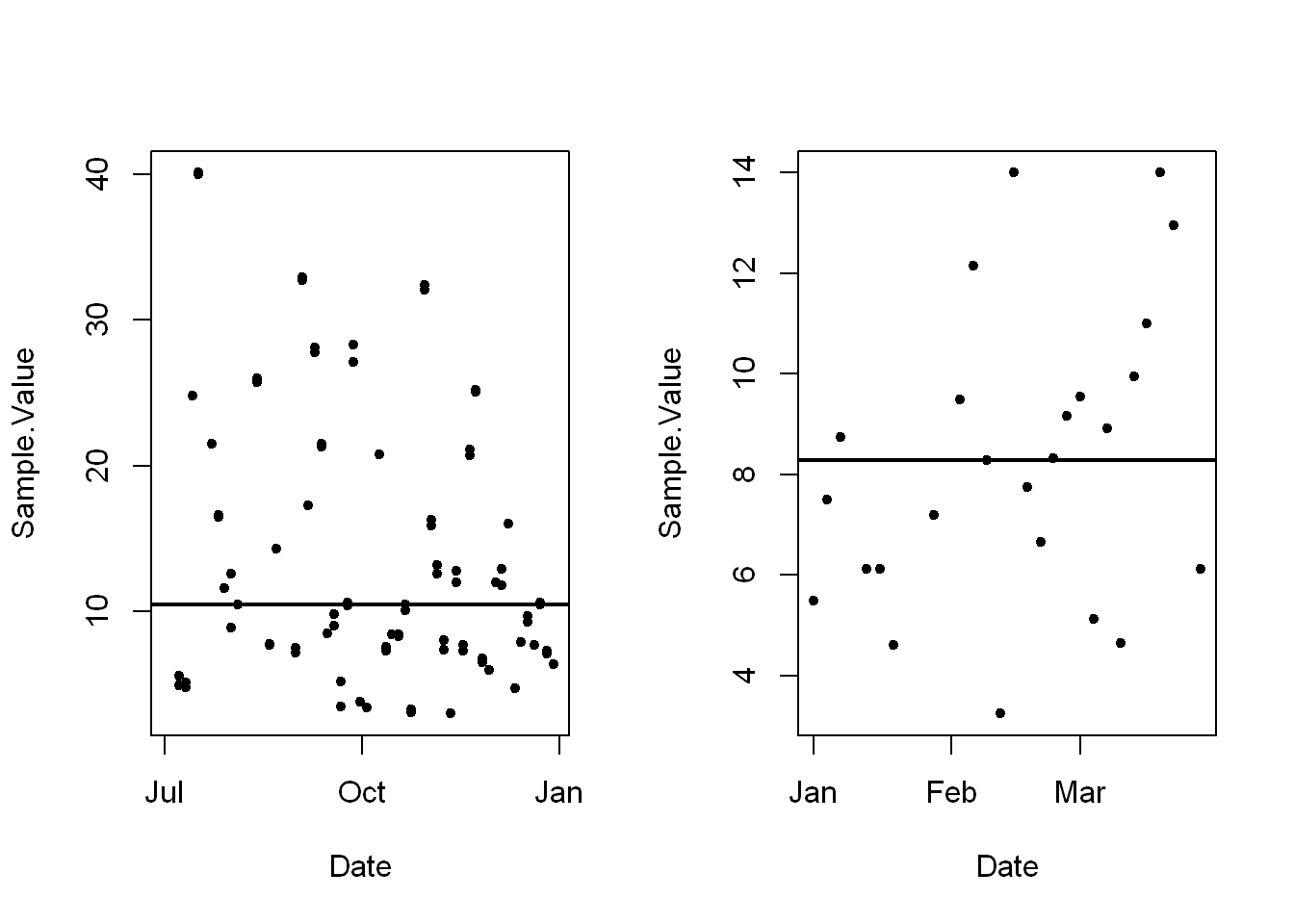
Calculate the ranges
As you can see from below that range0 includes range1 so it’s obvious the total range will be equal to range0
range0 <- range(pmosub$Sample.Value,na.rm=TRUE)
range0
[1] 3.0 40.1range1 <- range(pm1sub$Sample.Value,na.rm = TRUE)
range1[1] 3.25 14.00range <- range(range0,range1)
range[1] 3.0 40.1Set ylim
Let’s set the range to the ylim so we can have a more even comparison.
par(mfrow=c(1,2), max=c(4,4,2,1))Warning in par(mfrow = c(1, 2), max = c(4, 4, 2, 1)): "max" is not a graphical
parameterwith(pmosub,plot(Date, Sample.Value, pch=20, ylim=range))
with(pmosub,abline(h=median(Sample.Value, na.rm=TRUE), lwd=2))
# repeat for the second plot of 2012 data
with(pm1sub,plot(Date, Sample.Value, pch=20, ylim=range))
with(pm1sub,abline(h=median(Sample.Value, na.rm=TRUE), lwd=2))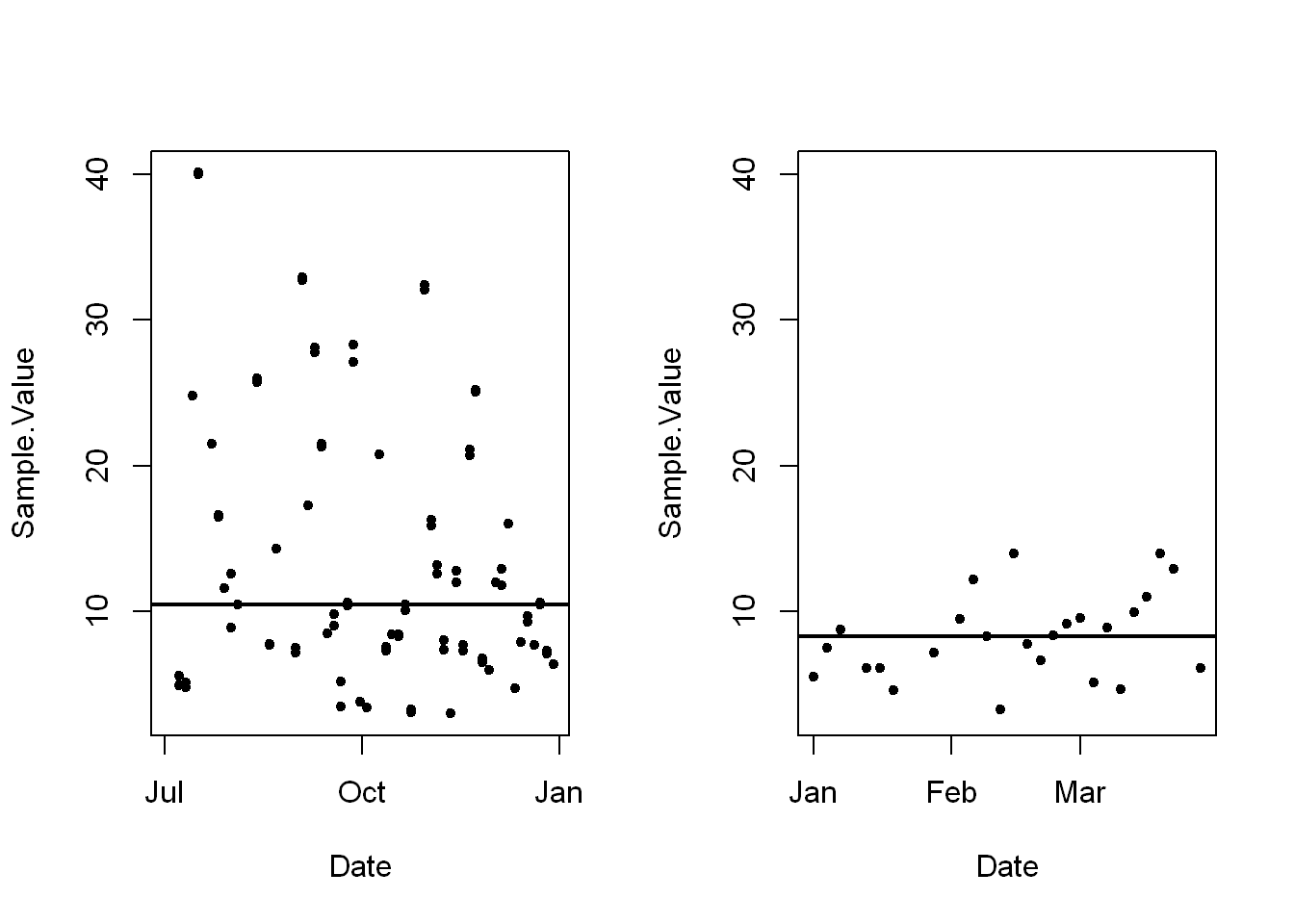
Average by State
We need to calculate the mean/average pollution levels by state, this could be done with group_by, aggregate… we’ll do it with tapply
- We’ll tapply a function “mean” to
- The Sample.Value for each state separately, basically we are calculating the mean of Sample.Value for each state as a group
- So that the output will be a list of numbers for each state’s mean, and a list of “char” for the names of each state
tapply mean/state
mn0 <- with(pm0_wnames,tapply(Sample.Value,State.Code, mean, na.rm=TRUE))
str(mn0)
num [1:53(1d)] 19.96 6.67 10.8 15.68 17.66 ...
- attr(*, "dimnames")=List of 1
..$ : chr [1:53] "1" "2" "4" "5" ...head(mn0) 1 2 4 5 6 8
19.956391 6.665929 10.795547 15.676067 17.655412 7.533304 mn1 <- with(pm1_wnames,tapply(Sample.Value,State.Code, mean, na.rm=TRUE))
str(mn1) num [1:52(1d)] 10.13 4.75 8.61 10.56 9.28 ...
- attr(*, "dimnames")=List of 1
..$ : chr [1:52] "1" "2" "4" "5" ...head(mn1) 1 2 4 5 6 8
10.126190 4.750389 8.609956 10.563636 9.277373 4.117144 Summary
We see from the summaries that all 6 columns decreased since 1999
summary(mn0) Min. 1st Qu. Median Mean 3rd Qu. Max.
4.862 9.519 12.315 12.406 15.640 19.956 summary(mn1) Min. 1st Qu. Median Mean 3rd Qu. Max.
4.006 7.355 8.729 8.759 10.613 11.992 Create data.frame
Let’s separate the “char” from mn0 into the names of the states, and the integer list into their means and assign each to a new column in a new dataframe for both years. d1 has 52 entries, and d0 has 53
d0 <- data.frame(state=names(mn0),mean=mn0)
d1 <- data.frame(state=names(mn1), mean=mn1)
head(d1)
state mean
1 1 10.126190
2 2 4.750389
4 4 8.609956
5 5 10.563636
6 6 9.277373
8 8 4.117144Merge dfs
Let’s merge the two by State
mrg <- merge(d0,d1, by="state")
dim(mrg)
[1] 52 3head(mrg) state mean.x mean.y
1 1 19.956391 10.126190
2 10 14.492895 11.236059
3 11 15.786507 11.991697
4 12 11.137139 8.239690
5 13 19.943240 11.321364
6 15 4.861821 8.749336Same plot
We’ll be plotting both on the same plot so we’ll use plot() once and follow it with points()
Plot with rep()
- The first argument is rep(1,52). This tells the plot routine that the x coordinates for all 52 points are 1.
- The second argument are the Y coordinates which is the second column of mrg or mrg[,2] which holds the 1999 data.
- The third argument is the range of x values we want, namely xlim set to c(.5,2.5).
- This works since we’ll be plotting 2 columns of points, one at x=1 and the # other at x=2.
- Plot the second plot with minor changes one being: we start with rep(2,52)
- And the data will be the third column for the year 2012 mrg[, 3]
- No need to repeat xlim since it is set already
with(mrg, plot(rep(1,52),mrg[ ,2], xlim= c(.5,2.5)))
with(mrg, points(rep(2,52),mrg[ ,3]))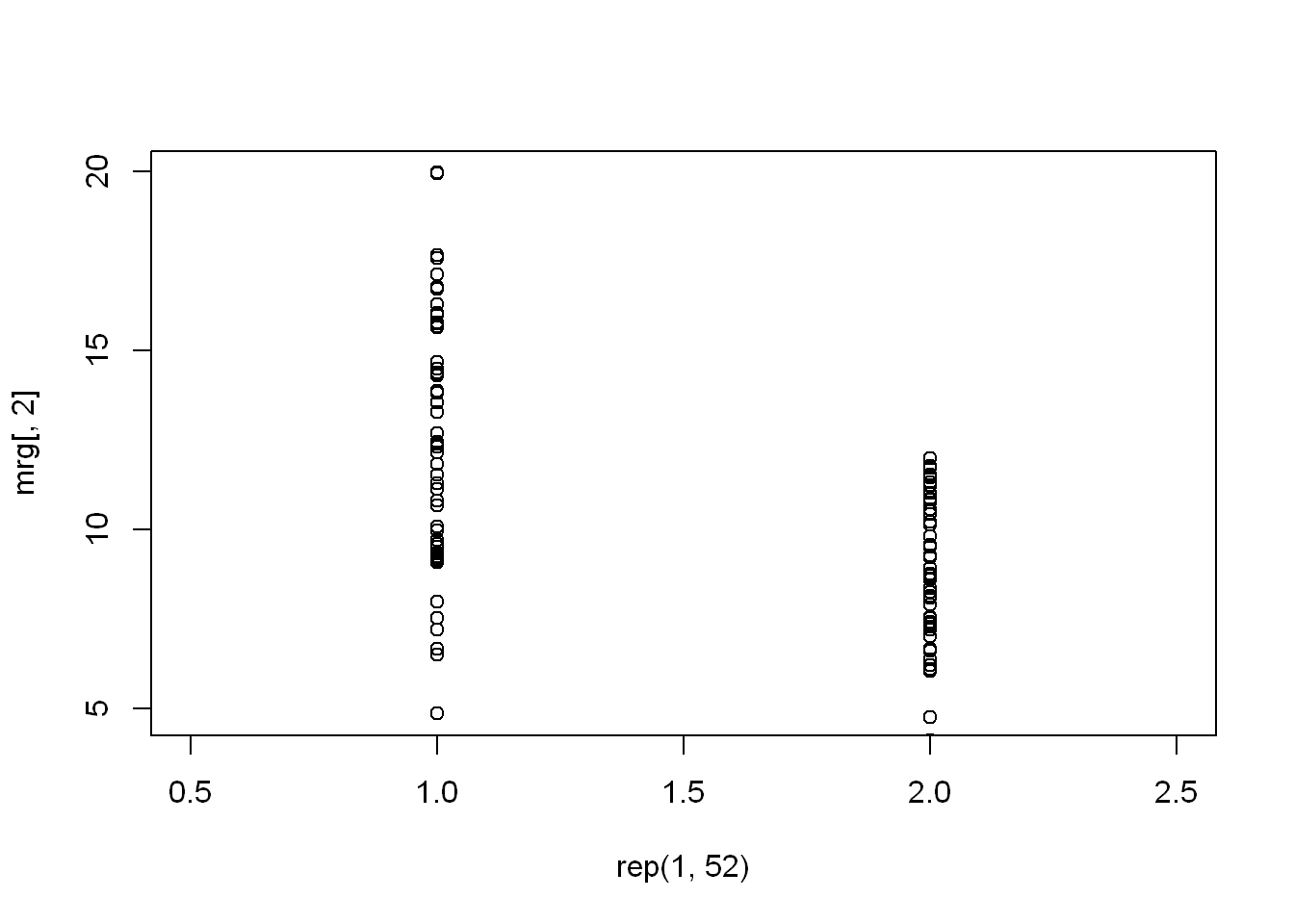
Connect Plots
Segments
We want to connect each state point from the 1999 plot with its corresponding point in the 2012 plot
We’ll use the function segments() with these arguments: - First 2 arguments are for the x and y of the left plot - Second pair of arguments is for the x and y of the right plot - As you can see the majority have a down sloping line except for a couple visible ones
with(mrg, plot(rep(1,52),mrg[ ,2], xlim= c(.5,2.5)))
with(mrg, points(rep(2,52),mrg[ ,3]))
segments(rep(1,52), mrg[ ,2], rep(2,52), mrg[ ,3])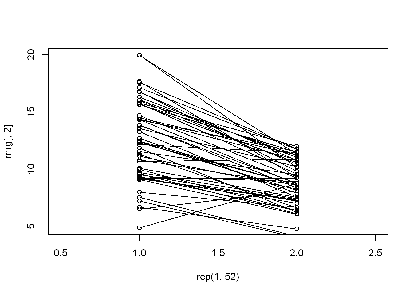
Extract higher means
The easiest way to extract the means that were higher in 2012 (or up sloping lines in plot), and we find that only 4 states had an increase in average emissions.
wentup <- mrg[mrg$mean.x < mrg$mean.y, ]
wentup
state mean.x mean.y
6 15 4.861821 8.749336
23 31 9.167770 9.207489
27 35 6.511285 8.089755
33 40 10.657617 10.849870Information
The sections below were not used but included as reference and additional information:
Vector to df
frame and wcol are two vectors, in order to save them with write_csv I will convert to df first then save
wcol_df <- data.frame(wcol)df to vector of strings
cnames_st <- toString(cnames) cnames_stconvert wcol_df to string as well
This is not needed for this process, included for information only.
wcol_st <- toString(wcol_df) wcol_stconvert df to string
This is not needed for this process, included for information only.
cnames_st <- strsplit(as.character(cnames_st),"|", fixed=TRUE) cnames_st